Continued Exploration
After reviewing the Netflix prize submission paper, we realized that there are quite a few nuances that our data plays to that the Netflix data doesn't. In order to get a grasp on the differences, we wanted to run some additional analysys. Firstly, we generated 30 random pairs of users and explored their shared ratings. In other words, are users rating the same movies so that we input from multiple people or are users fairly independent and only review different movies.
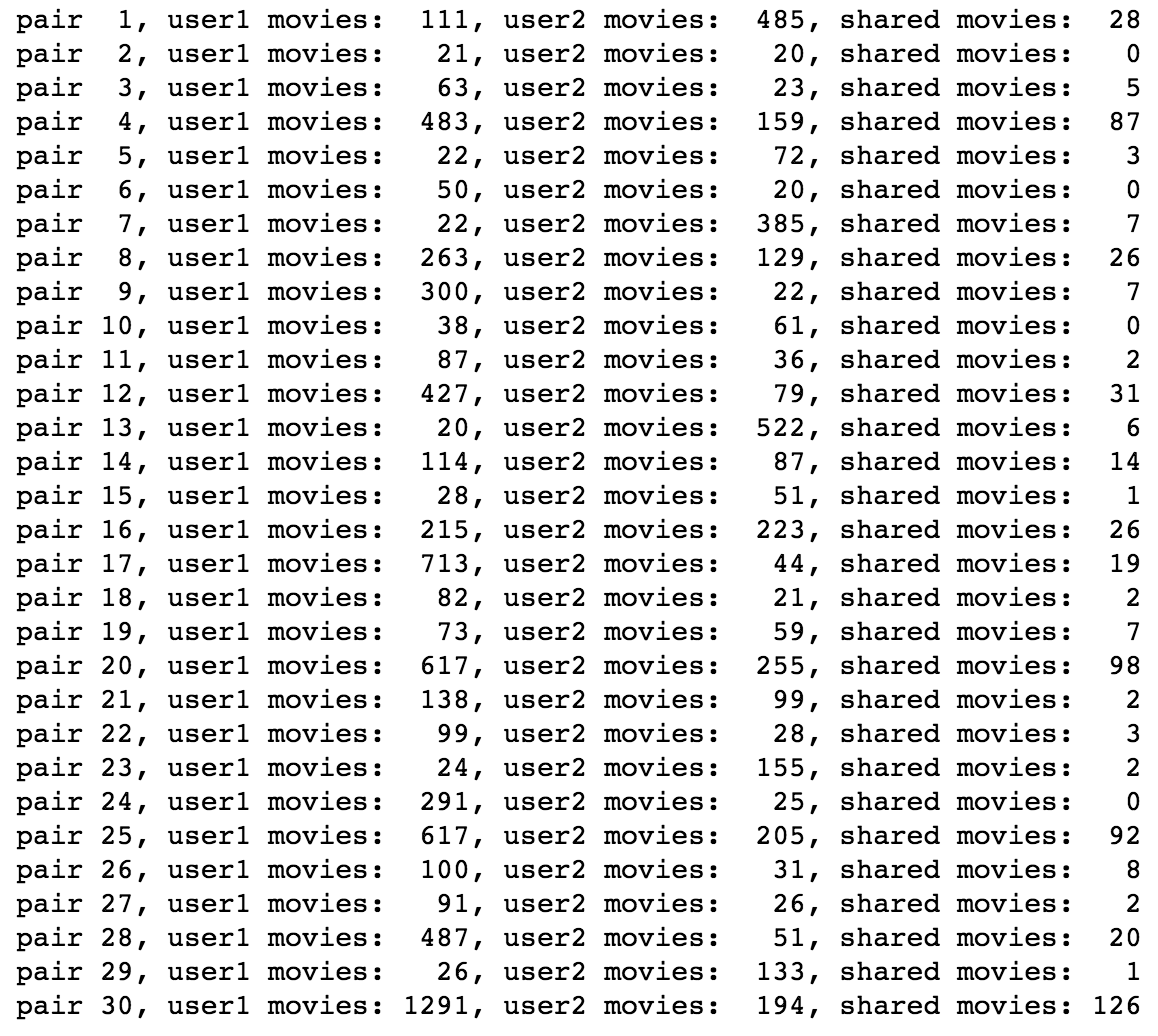
The result, as you can see in the image above, is that the mean number of shared movies from this sampling was just over 18 with a range from 0 - 126 shared movies. This is fairly concerning, from a prediction standput, as we can really only expect our model to perform so well, given that there isn't much overlap between reviews, users, and movies. Viewing the 30 random samplings in a histogram also shows us that the distribution isn't normal, but very skewed toward a bin of 25.2. The data is so skewed, in fact, that this bin is larger than all of the other bins combined.
Some other interesting differences between our dataset from MovieLens and the Netflix prize dataset:
1. The Netflix dataset has substantially more user input than the number of movies (users stating their preference, let's say). The exact opposite is true for our dataset, as the number of movies (~1700) is greater than the number of users submitting reviews (~1k). This is something we can expect to have an impact on our model.
2. The movies in the Netflix data have 20+ reviews per movie. In our dataset, we have nearly 50% of the movies with only 1 or 2 reviews. We can expect this to have an impact on our model as well.
3. The Netflix solution was also able to work with non-negative coefficients, which our model was not able to do. We believe this is because of the structure of our dataset (number of reviews per movie combined with a lack of overlap with reviews).
4. As a final note, the winning submission for the Netflix Prize blended over 100 models into their final solution. For the purposes of this project, and the dataset at hand, that would be hard to do since we don't have nearly as many predictors in our MovieLens dataset to create that many models. As a result, we are constrained to the number of predictors available in our dataset, unless we find a complementing dataset we can merge with our own that offers additional items we can leverage individual effects with.
Euclidean, Manhattan, and Pearson Correlation
Our first attempt at a model was distance based, relying on Euclidean, Manhattan, and Pearson correlation-based modeling. In a nutshell, these models compare 30 random pairs to determine how well of a fit we were able to create; a distance of 1 suggests a close fit while a distance of 0 is about as far away as you can get.
This approach, while a good starting point, wasn't particularly successful, as the mean distance for each of the models was: Euclidean- .195, Manhattan- .135, and Pearson- .207.
If you're interested in the code, give this pdf a view or visit the Notebook directly here.
User Effects and Item Effects and Blending them Together
Our second set of models took user effects and item effects independently and then blended. When taken independently, the models barely registered at the same level as our baseline models at .123 and .169. What's interesting, however, is that independently, the models performed pretty poorly but when combined, the score rose considerably to .254. We also took into account the possibility that portions of the dataset might be better served using the baseline prediction instead of our model. Combining all of these methods together (5 total models), and blending our models into a single solution, we still only had a score of .274.
If you're interested in the code, take a look at what's available here.
UV Decomposition
This seems to be a favorite topic among the data scientists of the World. We implemented UV composition across a portion of the dataset (let's say 5%), and the time that it took the model to run was severe. As a whole, training and predicting using our current dataset would have taken hours to process through the model. For this reason, we decided that although the findings would have been interesting to report here, the processing effort required train and test the model, with the results we had on a portion of the dataset, did not justify its continued use.
Our Winning Model!
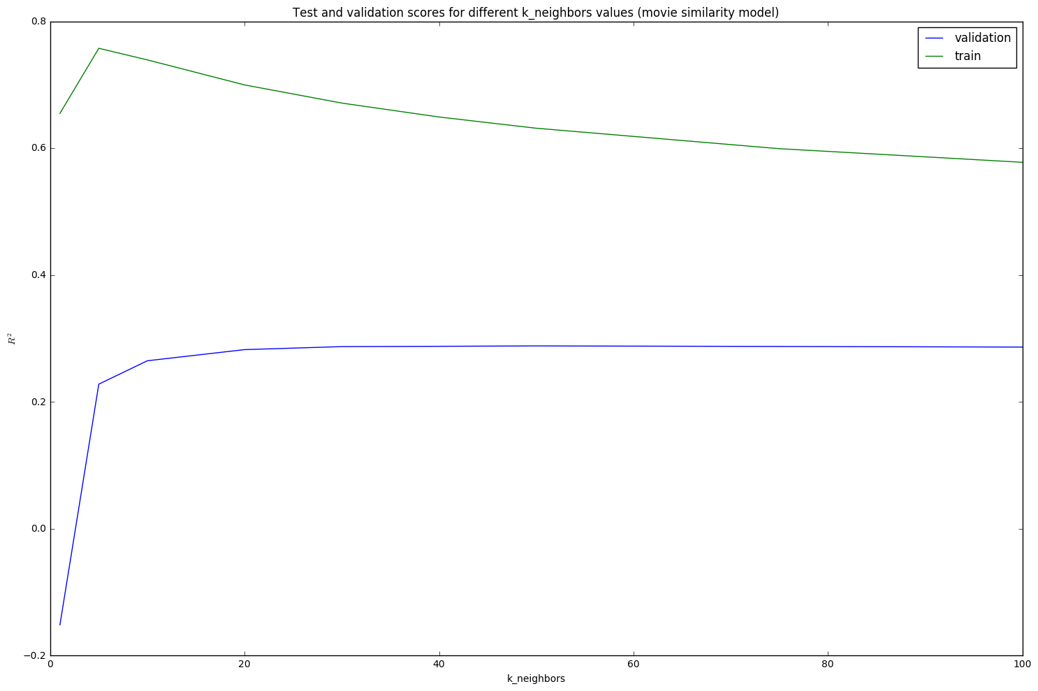
Our winning model for the project used blending of baseline values and k-nn (k=30) with item effects (movie similarity), where baseline values accounted for 7% of the datapoints. This model gave us our highest test score of .3045 and a Root Mean Square Error (RMSE) of .8776, taking 5 sec to initiate the effects, 1 min 21 sec to fit the data, and 11 min to score the model. If you'd like to take a look at our workbook, it's available here.
To build this Movie similarity model, we first removed all main global effects the same way we did for our baseline models. We subtracted the total rating mean, then we removed the movie effects and then user effects. As a result our utility matrix was the residuals after applying the baseline model. This allowed us to remove some scale differences in the way different users rate movies.
In our movie similarity model we predict the rating for a movie (movie_id) and a user (user_id) by:
1. Find k closest neighbors (k=40,50). For assessing item-item similarity, we calculated distance based on the mean squared error between items, using this equation:

This is the equivalent of using the inverse of Mean Square Error but adding a 1/α term: this introduces item support into the model, removes the possibility of producing an infinite loop for an answer, and gives us more confidence in the outcome of our prediction.
2. Since a relatively large number of movies have a low number of ratings (1-3), some of the movies have zero neighbors, in this case we use a baseline prediction (in 6.9-7.2% of the cases for the test set) in order to adjust our model for best fit.
Evaluating our Model
Now that we have the model that seems to best represent our dataset, let's go through the process of understanding how to effectively rate a recommendation engine. If you think back to the approach page, here are the areas we need to analyze our model, along with how these areas are typically analyzed (even if we don't have the ability to explore the model this in depth for the project, it's good for us to go through the motions of understanding next steps toward implementation):
1. User Preference- typically determined by user interviews and surveys. Simply posing the question, "which model do you prefer?" and measuring the experience of the user during the session
- This process is out of scope for the project but a very interesting and essential test of any model - let's run this by users and see if their gut reactions and feelings/preferences match what the data are telling us.
2. Prediction Accuracy- normally measured with R^2 or a similar error explanation term, this can also take into account the % of movies that were accurately predicted for the test set (within a given margin).
- In our case, let's compare our performance against the baseline, with regard to scoring. The baseline models, which leverage the mean for prediction, scored .125 and .174 and, when blended together, .259. Our model improves the prediction rating with a score of .309.
- Next question - were the gains worth the processing time and effort to build and implement the model? When we look at processing time for the models, let's take the blended baselines for comparison, which took 43.51 sec to fit. Our winning model took nearly double the time at 80.71 sec, to come in at 19% raw improvement for the score. In reality, the only way we can truly test if this is gain was worthwhile is to lean upon the first point and test how improved the feedback is for the time to fit. From our perspective, however, the gain is justified for an increase of 37 seconds to fit.
3. Coverage- measured by the percentage of all items that can ever be recommended given our dataset.
- This is a very interesting metric for a recommendation engine. When reviewing previous work in this field, we realized fairly early that the best way to improve coverage is to leverage a series of models to predict different stages of the dataset. For instance, if a part of the dataset falls well outside of a single model, we can blend a few models together to best represent the data. In our case, this is most apparent by substituting the baseline model when movie reviews are lacking for a particular title.
- We also found other sources that encouraged us to try throwing out the outliers of the dataset that were giving us trouble. For instance, if we know a couple of movies are not commonly watched or enjoyed, we can simply refuse to make recommendations for them or with them. This would lower the percentage of the dataset our model would cover but would likely increase the accuracy of the movies we did recommend. In our case, however, we elected to increase coverage to 100% as we decided that this project would be best served by building a model that predicts a movie regardless of the prior information we may have on it.
4. Confidence- (the system’s trust in its recommendations or predictions, which can grow with the amount of data it has to work with)
- Typically measured by a confidence interval of how likely a prediction is to be true. In our case, our model's score is fairly low, due to the nature of the dataset in question, so our confidence in the accuracy of our predictions is not very high
- However, it's important to note that this confidence interval will increase for any given model as more reviews are added to the system. In our case, however, we use a movie similarity model, which we can expect to raise our confidence slower than a review based model, for instance. Movies tend to take longer to produce and release than reviews take to create and submit. If we see an uptick in sequental films (read: Disney... make us some more Star Wars movies!), we would expect our confidence to improve quicker than the addition of Indie films, which are designed, by nature, to be different than what already exists in the marketplace.
5. Trust- (the user’s trust in the system’s recommendations, which may lead us to introduce prior beliefs to lead the system to recommend “safer” options for users so that it is “right” more often than not)
- This is another metric that is best tested with users and is therefore out of scope for this project.
6. Novelty- (recommendations for items that the user did not know about)
- Novelty is an unexpected jewel from a recommendation engine. In our case, we can expect our model to be more apt to recommend films that may be less known due to the number of movies that lack reviews. Our model focuses on the similarity of movies using nearest neighbor, so the possibility of novelty is much higher than a model that errs on the side of positive reviews.
7. Serendipity- (how surprising the successful recommendations are to users)
- Best measured through user testing as well
8. Diversity- (a measure of item-to-item similarity – recommending the same movie a user likes, for instance, isn’t particularly helpful)
- This is a measure that we were not able to test during this project. To perform a measurement of diversity, we would want to make a prediction that is not a movie that the user has previously seen, which would require additional data added to our dataset. This is something that would be really helpful to complete the model as we could begin to add user driven data to improve the accuracy of our predictions and, more importantly, not recommend those films the user has already seen.
9. Utility- (the expected utility of the recommendation – does this recommendation engine result in the service being used more, for instance)
- Measuring this recommendation engine property gets tricky without being implemented within a site. If we were to approach the fit of this model in this manner, we could leverage A/B testing and measure if there is an increase in usage for our service following its implementation.
10. Risk- (minimizing risk in recommending items)
- We did not incorporate risk mitigation within our model (only recommending highly reviewed titles, for instance). For the purposes of this project, we focused on recommending based upon movie similarity but we could definitely look at incorporating sentiment analysis in a later iteration that would prioritize recommendations for those movies that had more positive reviews.
11. Robustness- (the stability of the recommendation in the presence of fake information)
- Not tested and considered out of scope for this project.
12. Privacy- (no disclosure of private information from the user)
- We score a whopping 100% in this category. All user information was constrained to userid number and our dataset didn't contain user viewing habits. This is definitely an area you would need to be careful with if your recommendation became more user-based, however.
13. Adaptivity- (how well the model adapts to changing title availability and trends in preference)
- This is definitely an area that the model should be robust in. We have a sneaking suspicion that reviews tend to trail off the older the movie becomes (until reaching classical status, of course). The ability for a model to adapt to this kind of trend analysis would be ideal and it's also an area we did not incorporate into the model.
In summary, user preference, trust, novelty, and serendipity are all aspects that are best measured through user interaction and testing. Following this project, it would be best to establish a user testing session for the model to garner this feedback in order to perform a full review of the fit of our model for actual usage. Overall, however, we're rather pleased with how well our model performed given the challenges of the dataset.
Continuing our findings
To continue working through this dataset to find the ultimate model, we should consider the following approaches:
1. Focus on recommending movies that are higher rated and have more ratings- This entails introducing a prior into the model that would take our X-number of nearest neighbors and recommend the title that is highest rated or has more overall ratings. We believe that this would help improve prediction accuracy and user preference but it would most likely come at the price of novelty. The higher rating aspect of this would require the introduction off additional data, however, or the introduction of sentiment analysis on reviews/review titles.
2. Continued blending and binning- The winning Netflix prize model used over 100 models to craft the right solution. If we continue to leverage a variety of models and continue to introduce additional aspects of item support and priors, we may begin to see our model perform at a level worth implementing in the real world. Afterall, the advice from that team is to keep trying different approaches until you hit the right one!
3. Remove additional global effects- Just as we pulled out user and movie effects to build our models, we could continue doing the same process with actors, directors, genre, and more. We could emulate the rating using temporal information (ratings will decline as movies get older, for instance). This process could reveal some interesting information for our modeling process.
4. Try reducing the coverage of the model to improve user preference and trust- One approach we could use is to throw out movies that lack reviews or are truly outliers. By restricting the coverage of our model, we can remove the datapoints that produce the greatest error to our model. For our MovieLens dataset, however, this would mean losing nearly 50% of the movies in our database, simply to have 3 or more review per each film. We would need to make sure that the gains would justify the reduced coverage.
That concludes our project! THANK YOU for taking the time to look at our project and review our model. If you are interested in seeing our work, please visit our github page. And if you have specific recommendations on how to improve the model in the future, please feel free to comment on the repo! We look forward to hearing from you!